Is Particle Physics in Apache Beam a terrible idea?
Introduction
I usually work with apache beam, for work so I thought I’d stretch it a little further and use it for something outside it’s wheel house and see how bad it would be and write a simple 2d particle simulation processed with apache beam.
Why is this a bad idea? On a very cursory glance it seems like Beam handles parallelism for us, so it should be easy right? And it’s true, Beam is really good at trivially parallel processing tasks, the kind that makes up the bulk of Extract Transform and Load jobs in every enterprise you can think of. Where as our particle simulation is not trivially parallelisable, calculating the the new position of any particle requires knowledge of all of the others within the simulation.
Background
Right, so for our simulation we are going to solve the n-body problem, i.e. we have some number of point masses orbiting each other. The only interaction we will simulate is gravity. For simplicities sake, we’ll allow particles to move through each other (We could add a potential to give them size, something like a Lennard-Jones, but that’s not what where here to break)
I’ll also borrow a trick actual scientific computing and enforce periodic boundary conditions. Bascially we simulate a finite size box, and if one of our point masses goes out of one side, it will come back in the opposite side. This allows use fake infinite size, without needing infinite bits of precision (assuming our simulation is big enough to avoid self interaction)
We’ll also take some liberties with constants in our simulation, all lengths are unitless, the gravitiational constant is 1, every particle has the same unit mass, we will use a timestep of 1s, and interactions beyond a certain distance will be assumed to be 0. We also won’t choose our initial particle velocity from a distribution each particle will start stationary, and I’ll rely on the box being dense enough that something interesting will happen.
This might seem like a useless simulation, but even swapping the gravitational potential for the Lennard-Jones potential has been used in physics as an analogue for some surprisingly complex systems.
So the basic algorithm is as follows:
- Choose some initial positions for N particles
- For each of the N particles, find the M neighbours within an interaction cut-off
- For each of those neighbours, calculate the force it exerts on our particle.
- Sum all the forces on our particle, and move it a small amount in that direct.
- If we’ve done less than the required number of steps go back to 2.
Limitations - Loops?
So right off the bat we run into a limitation, Apache Beam can only process Acyclic graphs. So any processing procedure we come up with cannot have any loops in it. Which given the nature of our algorithm above is a bit of an issue. To work round this we’ll take inspiration from gcc and it’s --fun-roll-loops optimisation option and unroll the main loop into distinct processing steps. Now, if you think this would make a horrific graph, you would be right. See the following:
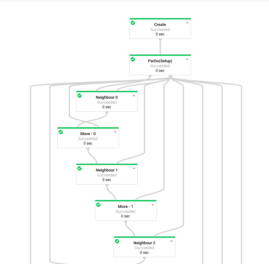
Now this graph looks worse than it is, I had a shared system configuration object which I was using as a side input. This also lead to Beam taking for ever to generate the graph. I refactored this away, as the steps and number of particles are effectively static anyway.
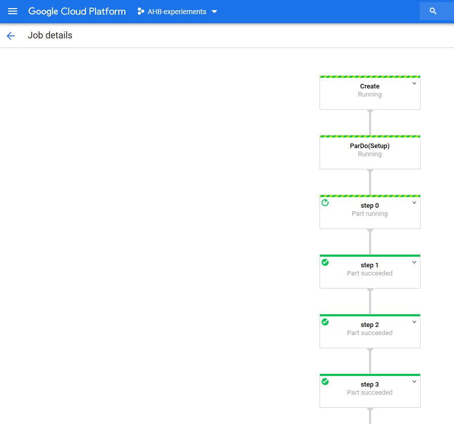
How does it Run?
Terribly. How terribly? Over 10 minutes for 10 steps using 1000 particles in 10x10 simulation. The directRunner actually outperforms Dataflow on this particular pipeline, presumabily because it keeps everything local and in memory. This will only work for small systems though where as the Dataflow should scale… right? Probably not, the main limiting factor is a our poor algorithm, that involves knowing about everything else.
Can we do better?
Probably. Now this isn’t how any sane Molecular Dynamics simulation package would calculate this. Typically long-range forces such as electrostatic interactions, can either make use of something like Particle Mesh Ewald to speed up this calculation, or use a cut-off beyond which the force is assumed to be 0. But that’s a bit beyond what were trying do here. What we can do instead is break our simulation cell into areas, group the charges within one of the area’s calculate the forces on those. This does inherently limit our scaling to the number of regions we divide the simulation into. But then it reduces the number of all particle interactions we have to calculate. This gets our run time down into the single minute run times for the same options as above, which is acceptable.
Summary
So what was the point of this? Mainly probing the limits of what a apache beam can do, or even what it was designed to do. If there had to be a take away message here it would be try and reduce the size of the side inputs, materialising these can be pretty expensive, as in our first example.